TL;DR — I packaged the entire ViT → Embedding → Fusion → Llama → Pooling pipeline into a single ONNX graph, lowered it to one FP16 TensorRT plan, and served it on Triton with three model instances and a 3 ms dynamic batcher. No conditional logic for text-only vs. image+text — every request runs the ViT, and masked_scatter no-ops when there are no image tokens. On an RTX 6000 Ada the engine peaks at ~54 inf/sec at concurrency 8 with a p99 of 183 ms; pushing concurrency past 16 trades real tail latency for no throughput. Practical operating range is concurrency 8–16; beyond that, scale horizontally.
This is Part 2 of three. Part 1 covers the model architecture and the two serving strategies I considered. Here I'll walk through Plan A end to end — the export, the engine build, the Triton config, and what perf_analyzer had to say about it. Part 3 does the same for Plan B, the multi-engine BLS router.
Table of contents
- System
- Architecture recap
- The ONNX-friendly model wrapper
- Building the TensorRT engine
- Triton serving config
- Benchmarking with perf_analyzer
- Results
System
| CUDA | 12.8 |
| GPU | NVIDIA RTX 6000 Ada Generation |
| Triton image | nvcr.io/nvidia/tritonserver:26.02-py3 |
| SDK image (perf_analyzer) | nvcr.io/nvidia/tritonserver:26.02-py3-sdk |
For the rest of this post I'll keep shapes simple: one image tile and a fixed sequence length of 1024. The first ~256 token positions belong to the image, the remaining ~768 to text plus padding. Everything generalizes to the model's full envelope (six tiles, 10,240 tokens), but the diagrams and numbers are easier to follow at this size.
DEVICE = "cuda" if torch.cuda.is_available() else "cpu"
FIXED_SEQ_LEN = 1024
MODEL_NAME = "nvidia/llama-nemotron-embed-vl-1b-v2"

model = (
    AutoModel.from_pretrained(
        MODEL_NAME,
        torch_dtype=torch.float16,
        attn_implementation="sdpa",
        trust_remote_code=True,
    )
    .to(DEVICE)
    .eval()
)
model.processor.max_input_tiles = 1
model.processor.use_thumbnail = False
model.processor.p_max_length = FIXED_SEQ_LEN
Architecture recap
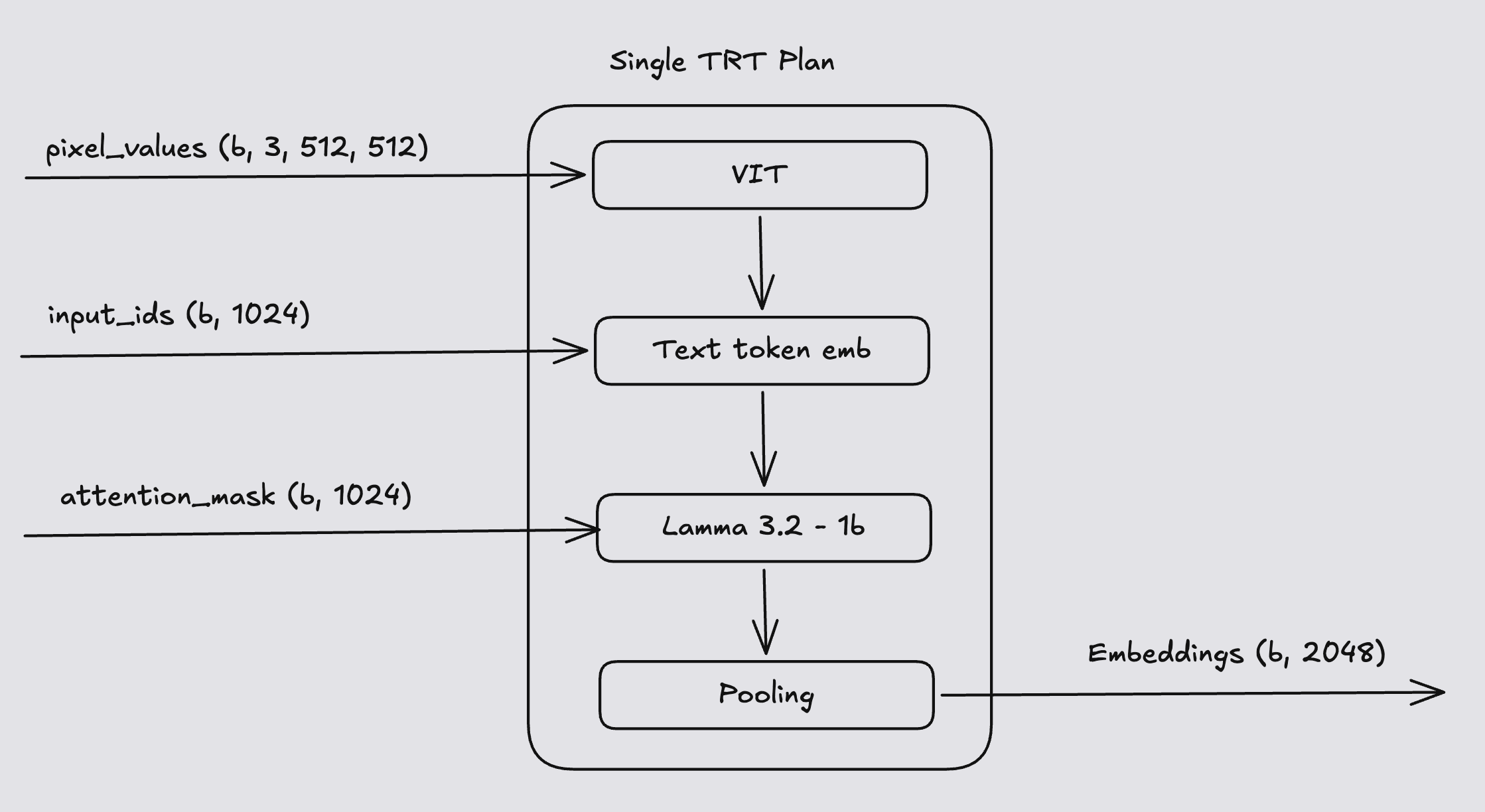
The whole pipeline is exported as one ONNX graph and lowered to one TensorRT plan. There is no runtime gate that decides whether to run the ViT — every request runs it. For image+text requests, masked_scatter rearranges the vision features into Llama's embedding stream wherever the input has img_context_token_id. For text-only requests, the client feeds a zero-filled pixel_values tensor; the preprocessor's attention_mask is already zeroed at the image-token positions, so the scatter is effectively a no-op and the LM ignores those rows.
The reason for this design is simple: ONNX doesn't trace conditional logic well. A graph that branches on whether an image is present is painful to export and either gets rejected by TRT or falls back to a slow path. So the engine path is identical for both modalities, and we pay a small "always run ViT" tax to keep the graph static.
The ONNX-friendly model wrapper
For torch.onnx.export to produce a single static graph, the forward pass has to be traceable end to end — no Python branching on tensor values, no data-dependent shapes. Below is the wrapper I used.
class NemotronModuleForOnnx(nn.Module):
    def __init__(self, model: nn.Module) -> None:
        super().__init__()
        self.model = model

    @staticmethod
    def embedding_pooling(
        ref_out: torch.Tensor, attention_mask_2d: torch.Tensor
    ) -> torch.Tensor:
        """Last attended token per row; ONNX-friendly (no batch-level branching)."""
        seq_len = attention_mask_2d.shape[1]
        rev = attention_mask_2d.flip(dims=[1])
        from_right = rev.argmax(dim=1).to(dtype=torch.long)
        last_idx = seq_len - 1 - from_right
        batch_idx = torch.arange(ref_out.shape[0], device=ref_out.device, dtype=torch.long)
        return ref_out[batch_idx, last_idx]

    def forward(self, pixel_values, input_ids, attention_mask):
        # Text embedding lookup
        input_embeds = self.model.language_model.get_input_embeddings()(input_ids)

        # ViT forward — runs unconditionally
        vision_embeds = self.model.extract_feature(pixel_values)

        # Fuse: splice vision rows into the input embedding stream
        batch_size, seq_len, hidden = input_embeds.shape
        input_embeds_flat = input_embeds.reshape(batch_size * seq_len, hidden)
        vision_embeds_flat = vision_embeds.reshape(-1, hidden)

        selected = input_ids.reshape(-1) == self.model.config.img_context_token_id
        input_embeds = input_embeds_flat.masked_scatter(
            selected.unsqueeze(-1).expand_as(input_embeds_flat),
            vision_embeds_flat,
        ).reshape(batch_size, seq_len, hidden)

        # Llama on the fused embeddings; attention_mask handles the
        # image vs. text-only distinction
        ref_out = self.model.language_model(
            inputs_embeds=input_embeds,
            attention_mask=attention_mask,
            use_cache=False,
        ).last_hidden_state
        return self.embedding_pooling(ref_out, attention_mask)
Two subtle things worth flagging. First, the pooling implementation deliberately avoids any batch-level "if left-padded vs. right-padded" branch — flip + argmax + gather traces cleanly and produces the same result HF's "last" pooling would. Second, the masked_scatter works for both modalities because the preprocessor sets attention_mask = 1 on image-token positions only when an image is actually present. Text-only requests have attention_mask = 0 there, so even though the scatter overwrites those rows with garbage from the zeroed pixel_values, the LM never attends to them.
Building the TensorRT engine
Once the ONNX file exports cleanly, I lower it to a single TRT plan with trtexec. Depending on your usecase you might want to have Fp32 for some layers ((LayerNorm, /div) etc,) to maintain precision, or use BFloat16 entirely. The optimization profile must include three batch points — min, opt, and max. TRT generates kernels tuned specifically for opt and extrapolates to other sizes within the legal range.
A quick word on choosing opt. This is the batch size the engine is most efficient at, so pick the size you expect to serve most often under steady load. With multiple model instances in Triton (see below), the per-engine batch is roughly concurrency / instance_count, so factor that in. I picked opt=16 for moderate traffic, with max=32 as the ceiling.
docker run --rm \
  --gpus "device=1" \
  --shm-size=2g \
  -v "/data:/data:rw" \
  nvcr.io/nvidia/tritonserver:26.02-py3 \
  /usr/src/tensorrt/bin/trtexec \
    --onnx=<your_onnx_path> \
    --saveEngine=<your_trt_plan_path> \
    --fp16 \
    --memPoolSize=workspace:8G \
    --minShapes=pixel_values:1x3x512x512,input_ids:1x1,attention_mask:1x1 \
    --optShapes=pixel_values:16x3x512x512,input_ids:16x1024,attention_mask:16x1024 \
    --maxShapes=pixel_values:32x3x512x512,input_ids:32x1024,attention_mask:32x1024 \
--skipInference| Flag | What it does |
|---|---|
--fp16 |
Build FP16 kernels (matches the model dtype). |
--memPoolSize=workspace:8G |
Build-time scratch — a bigger pool lets TRT consider more kernel variants. |
--minShapes / --optShapes / --maxShapes |
Dynamic-shape profile. opt is what gets tuned; min and max define the legal range. |
--skipInference |
Build only — don't run a sanity inference (we benchmark separately). |
Triton serving config
name: "model_1"
platform: "tensorrt_plan"
max_batch_size: 32

input [
  {
    name: "pixel_values"
    data_type: TYPE_FP16
    dims: [ 3, 512, 512 ]
  },
  {
    name: "input_ids"
    data_type: TYPE_INT64
    dims: [ 1024 ]
  },
  {
    name: "attention_mask"
    data_type: TYPE_INT64
    dims: [ 1024 ]
  }
]

output [
  {
    name: "last_hidden_state"
    data_type: TYPE_FP16
    dims: [ 2048 ]
  }
]

instance_group [
  {
    kind: KIND_GPU
    count: 3
  }
]

dynamic_batching {
  preferred_batch_size: [ 8, 16, 32 ]
  max_queue_delay_microseconds: 3000   # 3 ms
}
A few of these knobs are worth a closer look. max_batch_size: 32 matches --maxShapes on the engine — going higher would just be rejected. The preferred_batch_size list is ordered smallest-first so that under light traffic the batcher fires as soon as it can fill 8 rows; under heavier traffic it'll naturally grow toward 16 or 32. Including the TRT opt=16 value here matters: that's the size the engine is actually tuned for. The 3 ms max_queue_delay_microseconds is the upper bound on how long a request will wait for batch growth — a small amount of tail latency in exchange for noticeably bigger, more efficient batches. You can set it to 0 for pure latency mode if that's the priority.
The instance_group.count: 3 deserves its own paragraph. Three concurrent engines on the same GPU could achieve latency hiding to some extent Check out, which improves pipelining and keeps the GPU busier. The cost is 3× engine memory, which on a 48 GB RTX 6000 Ada is fine for this model but would not be fine for a much larger one.
Benchmarking with perf_analyzer
I benchmarked with NVIDIA's perf_analyzer from the matching -py3-sdk image. The sidecar container shares the server container's network namespace via --network "container:...", so localhost:8001 inside the sidecar is the server's gRPC port. Perf Analyzer
docker run --rm \
  --network "container:triton-nemotron" \
  -v "{your_path_to_model}:/work:rw" \
  nvcr.io/nvidia/tritonserver:26.02-py3-sdk \
  perf_analyzer \
    -m model_1 \
    -b 1 \
    -i grpc \
    -u localhost:8001 \
    --shape pixel_values:3,512,512 \
    --shape input_ids:1024 \
    --shape attention_mask:1024 \
    --input-data zero \
    --concurrency-range 8:32:8 \
    --measurement-mode time_windows \
    --measurement-interval 15000 \
    --stability-percentage 15 \
    --max-trials 4 \
    --percentile 99 \
    --collect-metrics \
    --metrics-url http://localhost:8002/metrics \
    -f /work/perf_analyzer_results.csv \
    --verbose-csv
The flag choices here are deliberate. -b 1 sets the client batch to one row per request — server-side dynamic batching does the actual coalescing, which is what I want to measure. --concurrency-range 8:32:8 sweeps in-flight requests at 8, 16, 24, and 32, covering below, at, and above the TRT opt/max range. Time-window measurement at 15 seconds is a better fit than count windows here because the sample size scales up with throughput rather than shrinking. A 15% stability tolerance is generous, but it has to be — the saturated regime has real queue jitter. --collect-metrics pulls GPU utilization, power, and memory from Triton's Prometheus endpoint and embeds them in the CSV alongside latency. And --input-data zero is fine because tensor content doesn't affect engine performance — the kernels run the same regardless of the bits.
Results
Concurrency sweep at BATCH=1, gRPC, 3 instances, OPT=16 engine, max_queue_delay=3ms:
| concurrency | inf/sec | GPU util | p50(ms) | p90(ms) | p95(ms) | p99(ms) |
|---|---|---|---|---|---|---|
| 8 | 53.86 | 0.951 | 148 | 168 | 170 | 183 |
| 16 | 47.93 | 0.992 | 333 | 484 | 512 | 523 |
| 24 | 45.13 | 0.995 | 524 | 715 | 798 | 910 |
| 32 | 43.98 | 0.996 | 727 | 735 | 741 | 1052 |
There are a few things to read out of this curve. Concurrency 8 is clearly the sweet spot for this engine — it produces the highest throughput (~54 inf/sec) and the lowest p99 (183 ms) at the same time. The GPU is already at 95% utilization there, which means each instance's effective batch size is well-fed but not yet over-saturated.
Pushing from 16 to 24 hits diminishing returns, and the math is straightforward. GPU utilization is already pegged at ~99%, so adding more in-flight requests can't actually speed anything up. Instead they pile up in the server queue and compute time grows because batch sizes start to exceed the TRT opt=16 regime — TRT extrapolates outside opt, and that extrapolation isn't free. The p99 reflects that exactly: 183 ms at concurrency 8 becomes 523 ms at 16, and 910 ms by 24. Throughput plateaus, latency tail grows roughly linearly with concurrency. Classic queue-fill behavior at saturation.
The takeaway is concrete. For this model on a single RTX 6000 Ada with three instances, the practical operating range is concurrency 8–16. Beyond that you trade significant tail latency for no real throughput gain. If you need to serve more than ~50 RPS, scale horizontally rather than pushing concurrency on a single GPU.
Part 3 takes the same workload and runs it through Plan B — the multi-engine BLS router that genuinely skips the ViT for text-only requests — and compares the numbers head to head.