TL;DR — The GPU utilization percentage is a poor signal on its own. It doesn't tell you whether you're compute-bound or memory-bound, and it doesn't tell you which part of the hardware is doing work. For transformer inference, what actually matters is Tensor Core utilization — how much of the matrix hardware is busy. Batch size grows the GEMMs that feed those cores, CUDA streams hide the latency between kernel launches, and model size determines how much any of that tuning can move the needle.
GPU utilization is one of those metrics that feels meaningful until you actually try to optimize it. A single percentage hides what the GPU is doing, how efficiently it's doing it, and whether changing anything will actually help. This post breaks down how GPU work is structured, what the different types of utilization mean, and what levers actually move the needle — using real profiling data from a Triton inference server setup.
Table of contents
- How the GPU Actually Executes Work
- Two main Types of GPU Activity
- Batch Size: What It Actually Does
- CUDA Streams and Concurrency
- Model Size Changes the Equation
How the GPU Actually Executes Work
Before utilization numbers mean anything, it helps to understand the hardware they describe.
An NVIDIA GPU is made up of Streaming Multiprocessors (SMs). Each SM is an independent compute unit containing CUDA cores, Tensor Cores (for matrix ops), shared memory, and register files. The A100, for example, has 108 SMs. When you launch a CUDA kernel, the GPU scheduler distributes work across these SMs.
Work is organized hierarchically: a kernel launch defines a grid of blocks, and each block contains threads. The block is the unit of scheduling — it gets assigned to an SM and runs entirely on that SM. Within a block, threads execute in groups of 32 called warps. A warp is the actual unit of execution: all 32 threads in a warp execute the same instruction in lockstep.
This matters because the GPU hides memory latency through warp switching. When a warp stalls waiting on a memory read, the SM switches to another resident warp and keeps executing. The more warps you have in flight per SM — the occupancy — the better the GPU can hide latency. Low occupancy means idle SMs, visible as poor utilization.
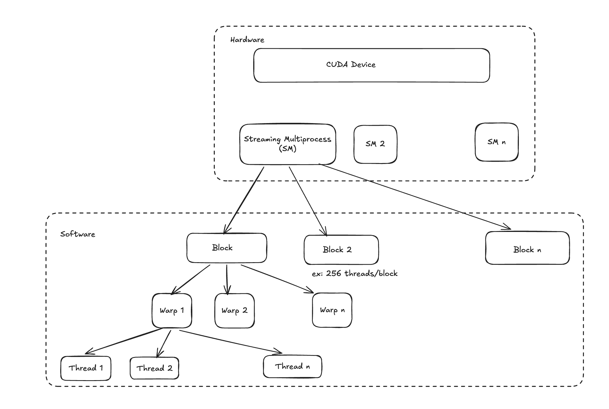 Source: Understanding Streaming Multiprocessors, Blocks, Threads and Warps in CUDA Programming
Tensor Cores are separate from CUDA cores and only activate for matrix multiply-accumulate (GEMM) operations. Most of the compute in transformer inference — attention, feed-forward layers — ends up as GEMM under the hood. Tensor Core utilization is the metric that actually matters for transformer workloads.
Two main Types of GPU Activity
When you open a profiler, GPU activity splits into two categories that look very different on a timeline.
Kernel Execution
This is compute. The GPU is running a kernel — doing actual math on the SMs. For ML inference, these kernels are mostly GEMM operations (matrix multiplications), attention computations, and elementwise activations. High kernel execution time means:
- SMs are busy
- Tensor Cores are being used
- The workload is compute-bound
This is what you want. The goal is to keep kernel execution time as high as possible and everything else low.
Memory Overhead (Memcpy)
This is data movement, not computation. To understand why it matters, it helps to know how memory is organized inside the GPU.
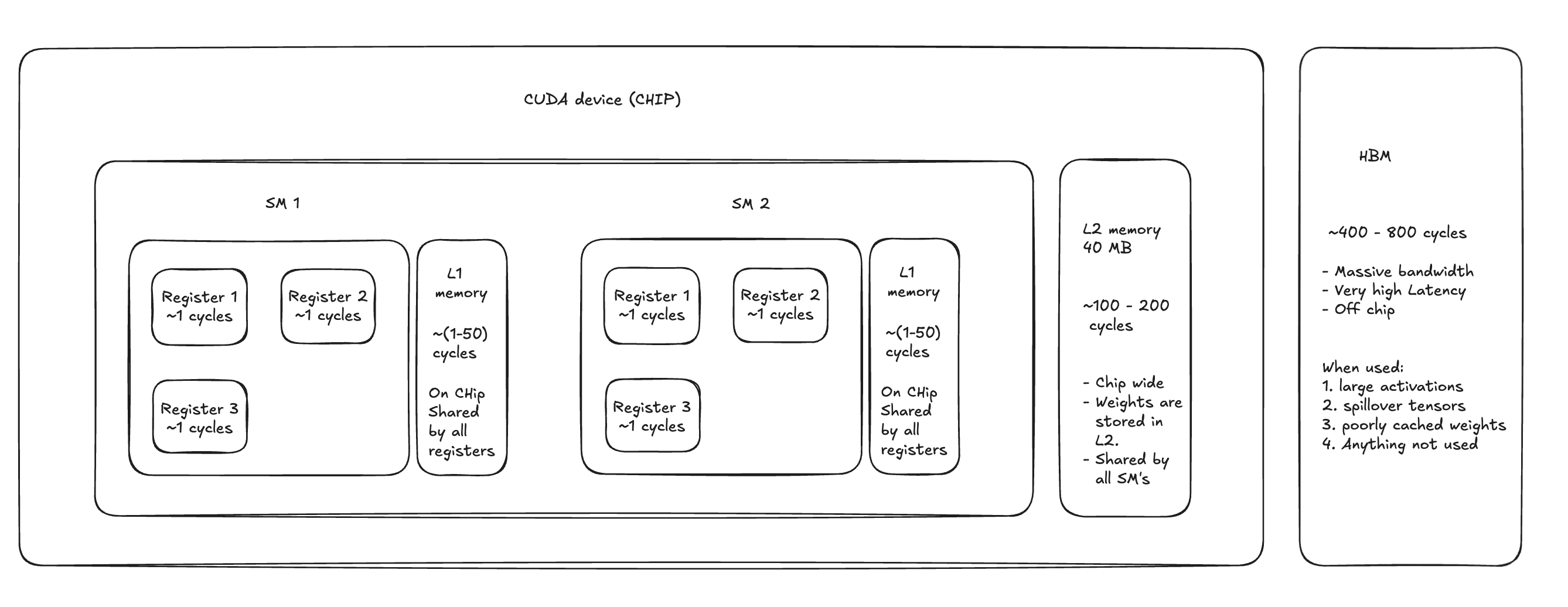
GPU cycles are the base unit of time on the GPU — one clock tick. A modern GPU runs at roughly 1–2 GHz, so a single cycle is about half a nanosecond. When a thread needs data, how fast it gets that data depends entirely on where that data lives.
Registers are the fastest storage on the chip, costing around 1 cycle. Each CUDA thread has its own private set, holding whatever values it's actively working with. There's no sharing, no contention — if your data is already in a register, access is essentially free.
L1 / Shared Memory sits inside each SM and is shared across all threads in a block. Access costs roughly 1–50 cycles depending on bank conflicts, and the capacity is small (48–192 KB per SM). It's commonly used to stage tiles in matrix operations or hold data that multiple threads in a block need to reuse.
L2 Cache is chip-wide — all SMs pull from the same 40 MB pool (on A100). It costs 100–200 cycles per access, but that's still far cheaper than going off-chip. Model weights for smaller models often live here after the first pass through the network, which is why cache-resident inference can be meaningfully faster.
HBM (High Bandwidth Memory) is the GPU's main memory — the "80 GB" you see on an A100 spec sheet. It's off-chip and slow at 400–800 cycles per access, though it compensates with enormous bandwidth (up to 2 TB/s). Large activations, tensors that don't fit in cache, and anything that hasn't been touched recently all end up here.
The further down this hierarchy a memory access falls, the longer a warp stalls waiting for data. Those stalls are what show up as gaps in a profiler trace. Three flavors of memcpy:
HtoD / DtoH — Host-to-Device and Device-to-Host copies. Data moving between CPU RAM and GPU memory over PCIe. These are slow and use copy engines, not compute units. In an inference pipeline, HtoD happens when you transfer input tensors to the GPU before the forward pass.
DtoD — Device-to-Device copies within GPU memory. Faster than HtoD/DtoH but still not compute. Happens during tensor reshaping, buffer reuse, and internal model operations like accessing cached weights. For small models that fit in L2 cache, DtoD latency can drop from 100–200 cycles down to 4–8 cycles — a meaningful difference when you're running high-throughput inference.
The profiler doesn't lie: if you see significant memcpy time, you're either moving data you don't need to move, or your compute kernels are too small to keep the GPU busy while the copies happen.
Batch Size: What It Actually Does
Batch size is the most common knob people reach for when trying to improve GPU utilization. Here's the actual mechanism.
A larger batch means larger input tensors, which means larger GEMM operations. Larger GEMMs give Tensor Cores more work per launch, which improves utilization. Larger batches, assuming asynchronous workflow, help hide memcpy latency — while a big kernel is running, there's more time for asynchronous memory operations to complete in the background.
But there are limits. If the model is already memory-bound — meaning the bottleneck is memory bandwidth, not compute — increasing batch size adds more data to move without proportionally increasing useful work. You can end up with higher utilization numbers while actually serving requests slower.
Smaller batches aren't always bad either. For compute-bound workloads with large kernels (common with transformer matmuls), even a small batch size say 4-8 can saturate the SMs. Multiple small kernel launches also benefit more from asynchronous execution — they can occupy all of the SM's. Kernel concurrency, however, is rare in large deep learning ops.
Too many small kernels, though, and you hit a different wall: kernel spawn overhead. Each kernel launch has CPU-side scheduling cost. Enough small kernels and the CPU can't keep the GPU fed, creating gaps in the GPU timeline.
CUDA Streams and Concurrency
A CUDA stream is an ordered queue of GPU operations. Operations within a stream execute in order; operations across streams can run concurrently if the GPU has spare capacity.
In a Triton inference server deployment, each instance may use multiple streams internally. Roughly model instances may share ~3–15 streams
Streams improve utilization when kernels do not fully occupy GPU resources. For example, if a kernel only uses a subset of streaming multiprocessors or leaves unused register or shared memory capacity, the GPU scheduler can launch kernels from other streams to fill those gaps. This improves hardware packing efficiency and helps hide latency from memory operations.
The catch: concurrency only helps when SM utilization is not already saturated. If your kernels are already using 95% of SM capacity, adding more streams doesn't increase throughput — it adds scheduling overhead, increases latency, and can cause cache thrashing from excessive interleaving. More streams on a fully loaded GPU is noise.
Model Size Changes the Equation
Model size determines whether batch size and stream counts matter at all.
Medium to large models Medium to large transformer models such as RoBERTa-large or multilingual embedding models typically generate large matrix multiplications even at small batch sizes. In transformer architectures, the effective matrix dimension is roughly (batch_size × seq_length, hidden_dim). Because sequence length can be large, even a batch size of one can produce sufficiently large GEMMs to keep Tensor Cores busy. In these cases, increasing batch size often provides limited additional benefit.
Sequence length can therefore influence utilization more strongly than batch size in transformer workloads, particularly because attention layers also introduce. O(seq_len)^2
Small models When model dimensions are small, the resulting GEMM operations may be too small to fully utilize the GPU. In these cases increasing batch size increases the matrix dimensions and produces kernels large enough to saturate more streaming multiprocessors.
Small models may also benefit from higher cache reuse because their weights and intermediate activations can fit more easily into the GPU's L2 cache. While device-to-device memory transfers are still limited by DRAM bandwidth, they are significantly faster than host-device transfers.
Deploying multiple small models on the same GPU can introduce additional CUDA streams and create natural concurrency. Because each model produces relatively small kernels that may not fully occupy GPU resources, the scheduler can interleave kernels from different streams, improving overall hardware utilization and partially compensating for small kernel sizes.
Understanding these mechanics is half the battle. The other half is reading what the profiler actually shows you — covered in